1. City of Austin Water Quality Master Planning - GIS Model David Maidment Francisco Olivera Mike Barrett Christine Dartiguenave Ann Quenzer CRWR - University of Texas

2. OVERVIEW zThe study area zDEM-based topographic analysis zGIS-based hydrologic analysis

3. The Study Area

4. LOCATION MAP

5. LAND USE

6. WATERSHEDS

7. EDWARDS AQUIFER

8. BMP’S

9. CONTROL POINTS

10. DEM-Based Topographic Analysis

11. USGS 7.5’ QUADRANTS OF THE AUSTIN AREA

12. DIGITAL ELEVATION MODEL (DEM)

13. HYDROLOGIC (RASTER-)GIS FUNCTIONS

14. FLOW DIRECTION zWater flows to one of its neighbor cells according to the direction of the steepest descent. zFlow direction takes one out eight possible values.

15. FLOW ACCUMULATION zFlow accumulation is an indirect way of measuring drainage areas (in units of grid cells).

16. STREAM DEFINITION zAll grid cells draining more than 250 cells (user-defined threshold) are part of the stream network.

17. STREAM SEGMENTATION zStream segments (links) are the sections of a stream channel connecting two successive junctions, a junction and the outlet, or a junction and the drainage divide.

18. WATERSHED DELINEATION zAll grid cells flowing towards a specific stream segment (link) constitute its watershed or drainage area. zThe watershed grid is then converted from raster into vector.

19. BURNING-IN PROCESS

20. DELINEATED STREAMS OF THE AUSTIN AREA

21. DELINEATED WATERSHEDS OF THE AUSTIN AREA

22. LOCATION OF CONTROL POINTS

23. GIS-Based Hydrologic Analysis

24. VECTOR AND RASTER REPRESENTATIONS OF THE TERRAIN Vector representationRaster representation The parameter represented can be land use, impervious cover, runoff coefficient, EMC...

25. IMPERVIOUS COVER VS. LAND USE

26. CURRENT IMPERVIOUS COVER

27. FUTURE IMPERVIOUS COVER

28. EQUATION FOR ESTIMATING ANNUAL LOADS zFor each land surface cell (30m x 30m): Load [M/T] = Precip [L/T] * Runoff Coeff * Mean Conc [M/L 3 ] *Cell Area [L 2 ] zLoad = Direct Runoff Load + Baseflow Load zUse weighted flow accumulation to get downstream loads zIn channel, load is adjusted for: ygroundwater recharge (flow and load decrease) ychannel erosion (load increase) zOverall loads are adjusted for BMP’s

29. DIRECT RUNOFF COEFFICIENT VS. IMPERVIOUS COVER Data obtained at small watersheds. One point per watershed per storm.

30. DIRECT RUNOFF COEFFICIENT VS. IMPERVIOUS COVER Data obtained at small watersheds. One point per watershed.

31. BASEFLOW COEFFICIENT VS. IMPERVIOUS COVER

32. EMC’S VS. IMPERVIOUS COVER zEstimation of individual storm EMC zEstimation of watershed EMC zRelating EMC’s with impervious cover

33. NH 3 CONCENTRATION VS. IMPERVIOUS COVER

34. TSS CONCENTRATION VS. IMPERVIOUS COVER

35. EMC’S VS. IMPERVIOUS COVER

36. VOLUME OF WATER PRODUCED IN EACH CELL Cell area Runoff coefficientPrecipitation (L/T) Volume of water produced by each cell (L 3 /T) Cell area (L 2 )

37. MASS OF POLLUTANT PRODUCED IN EACH CELL EMC (M/L 3 ) Mass of pollutant produced by each cell (M/L 3 ) Volume of water produced by each cell (L 3 /T)

38. VOLUME OF WATER LOST FROM EACH CREEK CELL OF THE RECHARGE ZONE L = cell size recharge zone Creek LV 2

39. FLOW LOST IN THE RECHARGE ZONE

40. FLOW / LOAD Volume of water or mass of pollutant produced by each cell Drainage area station The flow (L 3 /T) and load (M/T) are calculated with the weighted flow accumulation function, as the sum of the contributions from the upstream cells. The same process is followed for direct runoff and baseflow.

41. For each gauged location (USGS stations), observed flow and predicted flow (after recharge zone correction) were compared. For each station, and its corresponding drainage area, a correction factor corrcoef was defined in the following way: FLOW CALIBRATION

42. FLOW CORRECTION COEFFICIENT zFor the ungauged locations, the correction coefficient is extrapolated according to their impervious cover.

43. For each gauged location (USGS stations), observed load and predicted load (after recharge zone correction) were compared. For each station, it was assumed that the difference in load values was produced by channel erosion and a channel erosion coefficient was defined (Kg/yr/ft). LOAD CALIBRATION

44. LAND-GENERATED POLLUTANT CONCENTRATION

45. CHANNEL EROSION Apply the channel erosion equation to all ungauged watersheds. Add the channel erosion to the load at the stations.

46. CONSTITUENTS THAT INVOLVE CHANNEL EROSION zPure land contribution: BOD, COD, DP, NH 3, Cu, Pb, Zn. zLand and channel contribution: TSS, TOC, TP, TN.

47. Construction Load and BMP Effect

48. CONSTRUCTION LOAD x % of the area has a development amount of 100% 100 % of the area has a development amount of x% EMC(TSS) = 600mg/L Direct runoff coefficient = 0.5

49. LOCATED BMP’S DEFINED BY LOAD REMOVAL

50. LOCATED BMP’S DEFINED BY REMOVAL EFFICIENCY

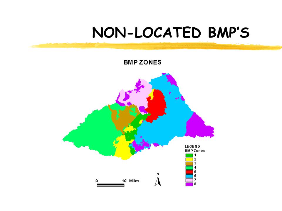
52. NON-LOCATED BMP’S

54. NON-LOCATED NON- DISCHARGE BMP’S Effective IC is used for calculating channel erosion.

55. CONCLUSIONS zThe goal of this research project was to determine current and future non- point source pollution loads in Austin streams. zThe model aims at being as flexible as possible: yThe BMP parameters and the EMCs can be easily modified and they do not require the analyst to recalibrate the model yModification of the current land use conditions, of the precipitation value used, or of the impervious cover/runoff coefficient relationships will require recalibration of the model zThe effects of both located and non-located BMP’s, and of construction activities were modeled. zCurrent flows matching observed flows at 17 USGS stations were determined zLoads were established for 122 sites (Environmental Integrity Index sites, USGS stations and mouths) within the study area.